Introduction to Logistic Regression - Sigmoid Function, Code Explanation

Logistic Regression is basically a predictive model analysis technique where the target variables (output) are discrete values for a given set of features or input (X). For example whether someone is covid-19 positive (1) or negative (0). It is a very powerful yet simple classification algorithm in machine learning borrowed from statistics algorithms.

 

Around 60% of the world’s classification problems can be solved by using the logistic regression algorithm. In this blog, we will explain what is logistic regression, difference between logistic and linear regression with python code explanation.

 

What is Logistic Regression?

 

Logistic regression is one of the most common machine learning algorithms used for binary classification. It predicts the probability of occurrence of a binary outcome using a logit function. It is a special case of linear regression as it predicts the probabilities of outcome using log function.

 

We use the activation function (sigmoid) to convert the outcome into categorical value. There are many examples where we can use logistic regression for example, it can be used for fraud detection, spam detection, cancer detection, etc.

 

Difference between Linear Regression vs Logistic Regression

 

Linear Regression is used when our dependent variable is continuous in nature for example weight, height, numbers, etc. and in contrast, Logistic Regression is used when the dependent variable is binary or limited for example: yes and no, true and false, 1 or 2, etc.

 

Linear regression uses the ordinary least square method to minimize the error and arrives at the best possible solution, and the Logistic regression achieves the best outcomes by using the maximum likelihood method.

 

In the 19th century, people use linear regression on biology to predict health disease but it is very risky for example if a patient has cancer and its probability of malignant is 0.4 then in linear regression it will show that cancer is benign (because probability comes <0.5). That’s where Logistic Regression comes which only provides us with binary results.

 

 

What is the Sigmoid Function?

 

It is a mathematical function having a characteristic that can take any real value and map it to between 0 to 1 shaped like the letter “S”. The sigmoid function also called a logistic function.

 

Sigmoid function

---

So, if the value of z goes to positive infinity then the predicted value of y will become 1 and if it goes to negative infinity then the predicted value of y will become 0. And if the outcome of the sigmoid function is more than 0.5 then we classify that label as class 1 or positive class and if it is less than 0.5 then we can classify it to negative class or label as class 0.

 

Why do we use the Sigmoid Function?

Sigmoid Function acts as an activation function in machine learning which is used to add non-linearity in a machine learning model, in simple words it decides which value to pass as output and what not to pass, there are mainly 7 types of Activation Functions which are used in machine learning and deep learning.

 

Code in Python

 

You can find the dataset here Dataset. First of all, before proceeding we first import all the libraries that we need to use in our algorithm

---

import numpy as np
import matplotlib.pyplot as plt 
from matplotlib.colors import ListedColormap 
import pandas as pd 
from sklearn.model_selection import train_test_split 
from sklearn.preprocessing import StandardScaler
from sklearn.metrics import accuracy_score
from sklearn.linear_model import LogisticRegression

---

After initializing all the libraries that we need in our algorithm know we have to import our dataset with the help of the pandas library and split our dataset into training and testing set with the help of the train_test_split library.

---

dataset = pd.read_csv(r'dataset.csv')
x = dataset.iloc[:,[2,3]].values
y = dataset.iloc[;, 4].values

x_train, x_test, y_train, y_test = train_test_split(x,y, test_size=0.2, random_state=0)

---

As we divide our dataset on the basis of train and test split know we have to scale our feature dataset with the help of StandardScaler library and apply logistic regression on the training set and check the accuracy sore with the help of accuracy_score library.

---

# Feature Scaling
sc = StandardScaler()
x_train = sc.fit_transform(x_train)
x_test = sc.transform(x_test)



# Fitting logistic regression to the training set
Classifier = LogisticRegression(random_state=0)
Classifier.fit(x_train, y_train)


# Predicting the test results
y_pred = classifier.predict(x_test)
print("Accuracy score: ", accuracy_score(y_test, y_pred))

# Accuracy score : 0.9125

---

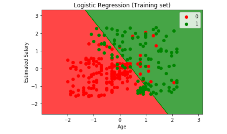
We have successfully applied logistic regression on the training set and see that our accuracy scores come 89%. So, if we take on basis of algorithm it is not so much worse for prediction. As we get the accuracy score of our model now we can see a pictorial representation of our dataset first we have to visualize the result on the basis of the training dataset.

---

X_set, y set = X_test, y_test
X1, X2 = np.meshgrid(np.arange(start = X_set[:, 0].min()- 1 ,

                               stop = X_set[:, 0].max() + 1,

                               step = 0.01),

                     np.arange(start - X_set[:, 1].min() -1,

                               stop = X_set[:, 0].max() + 1,

                               step = 0.01)),

plt.contourf(x1, x2, classifier.predict

    (np. array([X1.ravel(), X2.ravel()].T).reshape(X1.shape),

     alpha = 0.75, Cmap = ListedColormap(('red', 'green')))

plt.xlim(X1.min(), X1.max())

plt.ylim(X1.min(), X1.max())



for i,j in enumerate(np.unique(y_set)):

    plt.scatter(X_set[y_set== j, 0], X_set[y_set == j, 1],

      c =  ListedColormap(('red', 'green'))(i), label = j)          

plt.title('Logistic Regression (Training set)')
plt.xlabel('Age')
plt.ylabel('Estimated Salary')
plt.legend()
plt.show()

 

---

                                                                                    Estimated Salary Result(training set)

---

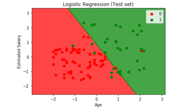
We plot a picture on the basis of age and estimated salary in which we bifurcate our result in a 0 and 1 value basis. In the same process, we apply for the test set and visualize our result how accurate our prediction is.

---

X_set, y set = X_test, y_test
X1, X2 = np.meshgrid(np.arange(start = X_set[:, 0].min()- 1 ,

                               stop = X_set[:, 0].max() + 1,

                               step = 0.01),

                     np.arange(start - X_set[:, 1].min() -1,

                               stop = X_set[:, 0].max() + 1,

                               step = 0.01)),

plt.contourf(x1, x2, classifier.predict

    (np. array([X1.ravel(), X2.ravel()].T).reshape(X1.shape),

     alpha = 0.75, Cmap = ListedColormap(('red', 'green')))

plt.xlim(X1.min(), X1.max())

plt.ylim(X1.min(), X1.max())


for i,j in enumerate(np.unique(y_set)):

    plt.scatter(X_set[y_set== j, 0], X_set[y_set == j, 1],

      c =  ListedColormap(('red', 'green'))(i), label = j)          

plt.title('Logistic Regression (Test set)')
plt.xlabel('Age')
plt.ylabel('Estimated Salary')
plt.legend()
plt.show()

 

                                                                                 Estimated Salary Result (Test Set)

---

Conclusion

 

The main concept regarding this blog is to explain logistic regression and simple explanation via python code. I think the above blog is very helpful for you to clear your doubts regarding logistic regression more blogs are on the way to stay tuned with us! Keep exploring Analytics Steps.